VOICES: Identidying Key Service Components
Introduction
The supplementary material for the paper looking at how different service components effect key clinical outcomes and health care use. This additional material demonstrates on a set of synthetic data, the data processing and analysis carried out for the paper “Identifying key health system components associated with improved outcomes to inform the re-configuration of services for adults with rare autoimmune rheumatic diseases: a mixed-methods study”.
Library
These are the packages that were used in the analysis of the data. Please note, the version numbers might be different, but the methods are still the same.
# packages for analysis and processing
library(tidyverse)
library(tidybayes)
library(brms)
library(lubridate)

# packages for figures and tables in this document
library(see)
library(ggridges)
library(reactable)

# Set the seed for reproducibility
set.seed(64327)
Load data
This loads in a dataset for the posterior samples from one of the models fit in this paper. This is from the multivariable analysis regarding the rates of Serious Infection. The data is arranged in a long format with the iter column linking draws from the posterior across the different parameters. Due to the link functions used in the brms package when fitting a negative binomial model, all coefficients for the mu value are on a log scale. For simplicity, coefficients for socio demographic features are not included in this dataset. As this is the case, the estimates retrieved from modelling these data will invariably be more certain than the real data.
df_SI <- read_csv("data/df_SI.csv")

head(df_SI)
# A tibble: 6 × 10
iter param Coef modelName fileName nVariables modelType DV SurveyLabel
<dbl> <chr> <dbl> <chr> <chr> <chr> <chr> <chr> <chr>
1 1 Interce… -1.83 m_nbinom… 2024_02… multivari… nbinom Seri… Intercept
2 2 Interce… -1.42 m_nbinom… 2024_02… multivari… nbinom Seri… Intercept
3 3 Interce… -1.71 m_nbinom… 2024_02… multivari… nbinom Seri… Intercept
4 4 Interce… -1.55 m_nbinom… 2024_02… multivari… nbinom Seri… Intercept
5 5 Interce… -1.60 m_nbinom… 2024_02… multivari… nbinom Seri… Intercept
6 6 Interce… -1.56 m_nbinom… 2024_02… multivari… nbinom Seri… Intercept
# ℹ 1 more variable: qGroup <chr>There are a few rows that aren’t needed for this demonstration, so the dataset will tidied up to make things easier to generate a synthetic dataset.
df_SI <- df_SI %>%
  select(iter, param, Coef) %>%
  spread(param, Coef) %>%
  select(iter, shape, Intercept, everything())

head(df_SI)
# A tibble: 6 × 10
iter shape Intercept AdviceandorLed CohortedClinic JointParaClinic
<dbl> <dbl> <dbl> <dbl> <dbl> <dbl>
1 1 0.125 -1.83 0.284 -0.0739 0.0142
2 2 0.156 -1.42 -0.206 -0.410 0.205
3 3 0.130 -1.71 0.0451 -0.109 0.168
4 4 0.130 -1.55 0.0996 -0.0932 0.0456
5 5 0.129 -1.60 0.173 -0.0493 0.105
6 6 0.154 -1.56 0.242 -0.151 -0.00568
# ℹ 4 more variables: LocalAAVpath <dbl>, OwnDayCaseUnit <dbl>, VascMDT <dbl>,
# WaitTimeNewWithinWeek <dbl>Now the posterior draws are in an easier format to use to make some synthetic data. As reported in the paper, different health boards had access to different service components. To this end, I will use the survey responses to generate a set of subjects for each synthetic board who has access to the respective components.
df_survResps <- read_csv("data/surveyResponses.csv") %>%
  # will help make things a little less confusing if I use a more descriptive label
  rename(Board = ID) %>%
  # need to tidy up the columns so they match the ones in the df_SI dataset
  mutate(
    # combine two responses
    AdviceandorLed = as.numeric(NurseAdviceLine | NurseLedClinic),
    # invert General Clinic value for Cohorted Clinics
    CohortedClinic = abs(GeneralClinic - 1),
    # Make columns for intercept and shape that are always on
    Intercept = 1,
    shape = 1
  )

df_survResps <- df_survResps %>%
  select(Board, colnames(df_SI %>% select(-iter)))

df_survResps
# A tibble: 17 × 10
Board shape Intercept AdviceandorLed CohortedClinic JointParaClinic
<dbl> <dbl> <dbl> <dbl> <dbl> <dbl>
1 1 1 1 0 1 0
2 2 1 1 1 1 1
3 3 1 1 0 0 0
4 4 1 1 0 0 1
5 5 1 1 0 1 0
6 6 1 1 0 1 1
7 7 1 1 0 1 0
8 8 1 1 0 0 0
9 9 1 1 0 0 1
10 10 1 1 1 1 1
11 11 1 1 0 1 1
12 12 1 1 0 0 1
13 13 1 1 0 0 0
14 14 1 1 0 1 0
15 15 1 1 0 1 0
16 16 1 1 0 0 0
17 17 1 1 0 1 1
# ℹ 4 more variables: LocalAAVpath <dbl>, OwnDayCaseUnit <dbl>, VascMDT <dbl>,
# WaitTimeNewWithinWeek <dbl>Generate Synthetic dataset
Create a dataset with 50 patients per service and add a column with a random iter value ranging from 1 to 2000 to retrieve a random draw from the posterior. Then I can combine the posterior draws dataset in order to get a value for the parameters in a negative binomial distribution. From this, I can then generate some synthetic data.
# create some patient data
df_patientData <- df_survResps %>%
  expand_grid(subj = 1:50) %>%
  mutate(iter = sample(1:nrow(df_SI), nrow(.), replace = T),
         subj = row_number())

# create a dataset that has the parameter values for each row in the df_patientData
df_params <- tibble(iter = df_patientData$iter) %>%
  left_join(df_SI)

# get the parameter values for each patient
for(i in colnames(df_params)[2:ncol(df_params)]){
  df_patientData[i] <- df_params[i] * df_patientData[i]
}

# create the mu parameter needed for the negative binomial dataset
timeMin <- .1
timeMax <- 24

df_patientData <- df_patientData %>%
  mutate(
    # calculate the mu value for the negative binomial parameter
    mu = exp(rowSums(across(c(Intercept:WaitTimeNewWithinWeek)))),
    # add in a random value for the time in study
    timeYears = round(runif(nrow(.), timeMin, timeMax), digits = 2)
  )
Simulate visit data
Now all the values are in the dataset, we can produce count data for the number of visits each patient had during the time they were in the study.
Demonstration
To show that this function behaves in the expected way, I have generated two datasets using the bespoke nbinomProcess function and the built in rnbinom function to generate two datasets using the same parameters. The exposure time will be kept constant to allow for an easier comparison to be made with the true distribution.
# set some parameters
N <- 1e6
thisMu <- 3.4
thisSize <- 10.3

# generate data using the rnbinom() function
df_rnbinom <- tibble(subj = 1:N,
                     nEvents = rnbinom(N, thisSize, mu = thisMu),
                     thisFunction = "rnbinom")

# generate data using the nbinomProcess() function
df_nbinomProcess <- tibble(subj = 1:N,
                           thisFunction = "nbinomProcess")
df_nbinomProcess$nEvents <- sapply(1:N, function(i){
  nbinomProcess(thisMu, thisSize, 1)
})
df_nbinomProcess$nEvents <- sapply(1:N, function(i){
  length(df_nbinomProcess$nEvents[[i]])
})

# create figure to compare
rbind(df_rnbinom, df_nbinomProcess) %>%
  ggplot(aes(nEvents, fill = thisFunction)) +
  geom_histogram(binwidth = 1,
                 position = "dodge") +
  geom_line(data = tibble(x = 0:max(c(df_rnbinom$nEvents, df_nbinomProcess$nEvents)),
                          y = dnbinom(x, thisSize, mu = thisMu) * N),
            aes(x, y),
            inherit.aes = F) +
  geom_point(data = tibble(x = 0:max(c(df_rnbinom$nEvents, df_nbinomProcess$nEvents)),
                           y = dnbinom(x, thisSize, mu = thisMu) * N),
             aes(x, y),
             size = 3,
             inherit.aes = F) +
  scale_fill_flat()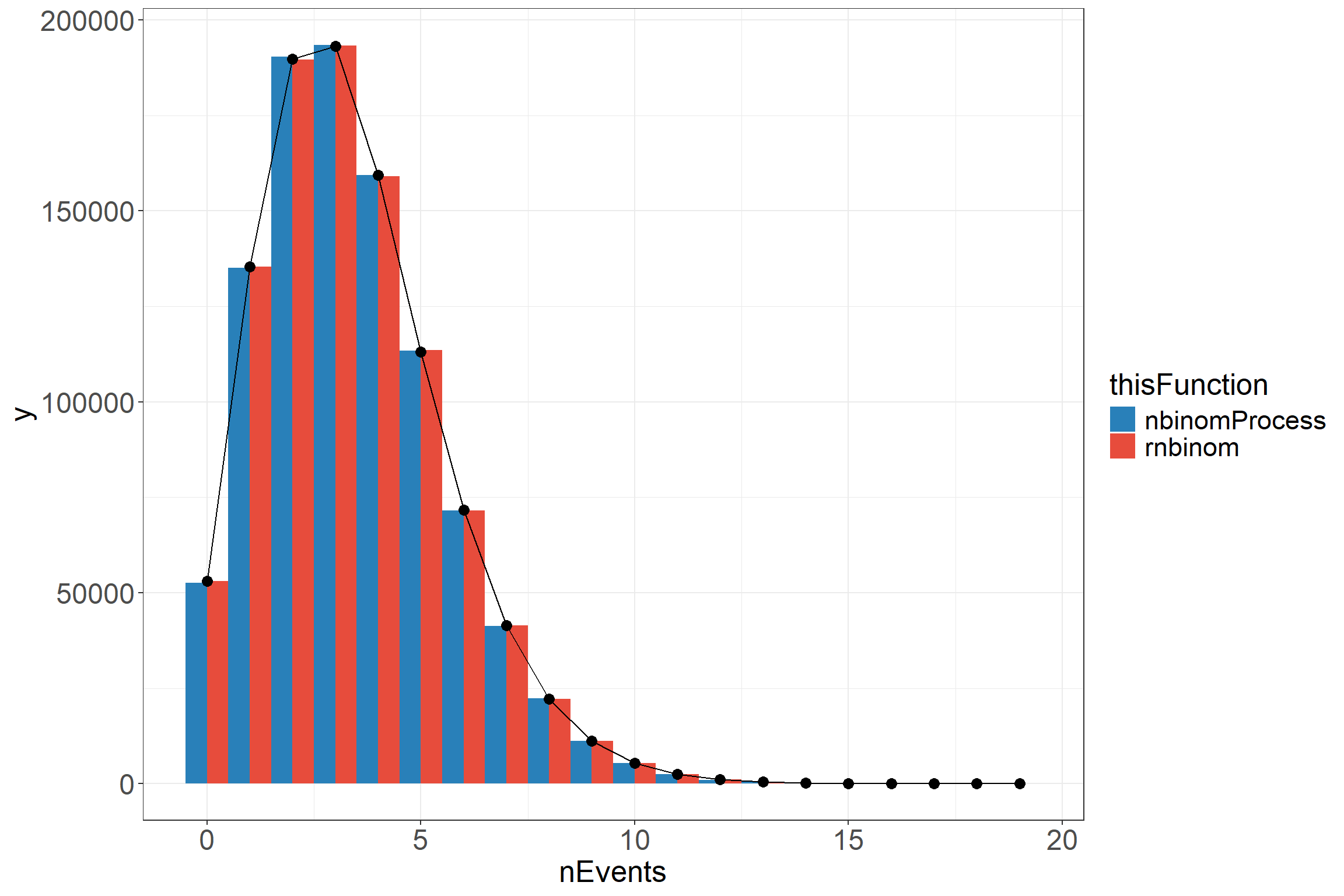
From the above, we can see that the functions produce very similar results that both match onto the true distribution with a high enough number of samples. The reason for the nbinomProcess function is to produce a number of events with time stamps to make data that looks similar to what would be available for analysis.
Create synthetic dataset
# generate a series of positive and negative events
# For the purposes of this dataset, I've made it so that everyone has 3 "negative" events
toBind <- t(sapply(1:nrow(df_patientData), function(i){
  time <- df_patientData$timeYears[i]
  genVisits(3, df_patientData$mu[i], df_patientData$shape[i] * time, time)
}))

# bind the data and unnest the list columns
df_patientData <- df_patientData %>%
  cbind(toBind) %>%
  unnest(c(posEvent, EventTime))
Format dataset
Now we have the event times, we can make the dataset look a touch more realistic.
# end Date of study to get index data for each patient
endDate <- as.Date("2020-10-31")

# function to convert between numbers and the data
ChangeTime <- function(og_date, thisYears){
  if(thisYears[1] < 0){
    sub <- T
    thisYears <- abs(thisYears)
  } else {
    sub <- F
  }

  # sort year value
  floorYears <- floor(thisYears)

  # sort month value
  thisMonth <- (thisYears - floorYears) * 12
  floorMonth <- floor(thisMonth)

  # sort day value
  thisDay <- thisMonth - floorMonth
  thisDay <- round(thisDay * 28)

  # have to do the months as days because it goes wonky with certain dates otherwise
  if(sub){
    og_date -(years(floorYears) + days(floorMonth * 28) + days(thisDay))
  } else {
    og_date + (years(floorYears) + days(floorMonth * 28) + days(thisDay))
  }
}

# format the dataset to look more realistic
df_patientData <- df_patientData %>%
  select(-c(Intercept, shape, iter, mu)) %>%
  mutate(across(c(AdviceandorLed:WaitTimeNewWithinWeek), ~ abs(.x) > 0),
         indexDate = ChangeTime(endDate, -timeYears),
         eventDate = ChangeTime(indexDate, EventTime)) %>%
  select(subj, indexDate, Board, timeYears, everything(), -EventTime)

# add in an mcon column which is based on whether the event was "positive"
# NB: The "Codes_X" variables are defined in the markdown document which can be
#     found in the github repository.
#     They are the same as the codes seen in the readME file for the repository.
df_patientData$mcon <- sapply(1:nrow(df_patientData), function(i){
  if(df_patientData$posEvent[i]) {
    sample(Codes_SI, 1)
  } else {
    sample(c(Codes_Cancer, Codes_CVD), 1)
  }
})

# Add in some other codes
df_patientData$ocon <- sapply(1:nrow(df_patientData), function(i){
  nOthers <- sample(0:5, 1)
  if(df_patientData$posEvent[i]){
    output <- sample(c(Codes_SI, Codes_Cancer, Codes_CVD), nOthers)
  } else {
    output <- sample(c(Codes_Cancer, Codes_CVD), nOthers)
  }
  paste(c(output, rep("NA", 5 - nOthers)), collapse = "|")
})

# tidy up the dataset
df_patientData <- df_patientData %>%
  separate(ocon, into = paste0("ocon", c(1:5)), sep = "[|]")

# show the dataset
reactable(df_patientData)
Please note, the ICD-10 codes that don’t relate to Serious Infection were sample from two other lists regarding Cancer and Cardiovascular Disease so these probably aren’t the most clinically valid. The extra codes are simply there to give an impression of what the real data looks like.
Modelling
Now we have a somewhat realistic dataset, we can model these data. The data needs to be processed so it is in a format that is amenable to being modelled. To do this, we need a single row per patient with a count of how many events of interest occurred (Serious Infections in this case), how long they were in the study for, and which services were available in their primary board of treatment. In the real data, we would need to check for the presence of ICD-10 codes relating to Serious Infection, but as this data is synthetic we already have a flag for rows where an ICD-10 code for Serious Infection was present. Another thing to consider is that the real data were drawn from inpatient records. As this was the case, in the original dataset there could be multiple rows for a continuous stay. When cleaning the real data, care has to be taken to avoid counting the same event multiple times due to patients being transferred during a single continuous stay. Fortunately here, we don’t have to deal with that, but this should be kept in mind when looking at real data of this sort.
df_modelData <- df_patientData %>%
  group_by(subj, Board, timeYears,
           AdviceandorLed, CohortedClinic, JointParaClinic, LocalAAVpath,
           OwnDayCaseUnit, VascMDT, WaitTimeNewWithinWeek) %>%
  summarise(SI_events = sum(posEvent))

reactable(df_modelData)
Run model
The model was fit using the brms library. All variables regarding the service components were entered as main effects. In the paper, additional parameters include Sex (deviation scaled), Age (median centered and decade scaled), Urban/Rural status (2 fold classification), and Scottish Index of Multiple Deprivation (as quintiles with 3 set as the baseline). Additionally, there was a random intercept for board of treatment to account for differences in base rates of Serious Infection. For this example, these haven’t been included. All coefficients regarding the service components (and the demographic features in the paper) were given a weakly informative prior of a student t distribution with a mean of 0, degrees of freedom of 3, and standard deviation of 1. A comparison between the prior predictions and posterior predictions can be seen by fitting the same model with the sample_prior argument set to "only".
my_prior <- prior(student_t(3, 0, 1), class = "b")

# A model that only samples the prior
# I've commented this out because it doesn't need to be run here
# but should you want to check the prior assumptions, this is the code you need
# m_nbinomn_priorOnly <- brm(
#   SI_events | rate(timeYears) ~
#     AdviceandorLed + CohortedClinic + JointParaClinic +
#     LocalAAVpath + OwnDayCaseUnit + VascMDT +
#     WaitTimeNewWithinWeek,
#   data = df_modelData,
#   family = negbinomial(),
#   prior = my_prior,
#   sample_prior = "only",
#   chains = 1,
#   iter = 4000,
#   warmup = 3000,
#   control = list(adapt_delta = .9)
# )

m_nbinom <- brm(
  SI_events | rate(timeYears) ~
    AdviceandorLed + CohortedClinic + JointParaClinic +
    LocalAAVpath + OwnDayCaseUnit + VascMDT +
    WaitTimeNewWithinWeek,
  data = df_modelData,
  family = negbinomial(),
  prior = my_prior,
  chains = 1,
  iter = 4000,
  warmup = 2000,
  control = list(adapt_delta = .9)
)
Compiling Stan program...Start sampling
SAMPLING FOR MODEL 'anon_model' NOW (CHAIN 1).
Chain 1:
Chain 1: Gradient evaluation took 0.00048 seconds
Chain 1: 1000 transitions using 10 leapfrog steps per transition would take 4.8 seconds.
Chain 1: Adjust your expectations accordingly!
Chain 1:
Chain 1:
Chain 1: Iteration:    1 / 4000 [  0%]  (Warmup)
Chain 1: Iteration:  400 / 4000 [ 10%]  (Warmup)
Chain 1: Iteration:  800 / 4000 [ 20%]  (Warmup)
Chain 1: Iteration: 1200 / 4000 [ 30%]  (Warmup)
Chain 1: Iteration: 1600 / 4000 [ 40%]  (Warmup)
Chain 1: Iteration: 2000 / 4000 [ 50%]  (Warmup)
Chain 1: Iteration: 2001 / 4000 [ 50%]  (Sampling)
Chain 1: Iteration: 2400 / 4000 [ 60%]  (Sampling)
Chain 1: Iteration: 2800 / 4000 [ 70%]  (Sampling)
Chain 1: Iteration: 3200 / 4000 [ 80%]  (Sampling)
Chain 1: Iteration: 3600 / 4000 [ 90%]  (Sampling)
Chain 1: Iteration: 4000 / 4000 [100%]  (Sampling)
Chain 1:
Chain 1:  Elapsed Time: 8.195 seconds (Warm-up)
Chain 1:                19.736 seconds (Sampling)
Chain 1:                27.931 seconds (Total)
Chain 1: summary(m_nbinom) Family: negbinomial
Links: mu = log; shape = identity
Formula: SI_events | rate(timeYears) ~ AdviceandorLed + CohortedClinic + JointParaClinic + LocalAAVpath + OwnDayCaseUnit + VascMDT + WaitTimeNewWithinWeek
Data: df_modelData (Number of observations: 850)
Draws: 1 chains, each with iter = 4000; warmup = 2000; thin = 1;
total post-warmup draws = 2000
Population-Level Effects:
Estimate Est.Error l-95% CI u-95% CI Rhat Bulk_ESS
Intercept -1.66 0.15 -1.95 -1.37 1.00 1750
AdviceandorLedTRUE 0.10 0.18 -0.25 0.45 1.00 1436
CohortedClinicTRUE -0.15 0.09 -0.32 0.02 1.00 1600
JointParaClinicTRUE 0.05 0.09 -0.14 0.21 1.00 2229
LocalAAVpathTRUE -0.13 0.10 -0.32 0.06 1.00 1728
OwnDayCaseUnitTRUE 0.11 0.11 -0.10 0.32 1.00 1581
VascMDTTRUE -0.14 0.17 -0.47 0.21 1.00 1562
WaitTimeNewWithinWeekTRUE -0.04 0.12 -0.29 0.21 1.00 1851
Tail_ESS
Intercept 1593
AdviceandorLedTRUE 1297
CohortedClinicTRUE 1514
JointParaClinicTRUE 1451
LocalAAVpathTRUE 1405
OwnDayCaseUnitTRUE 1630
VascMDTTRUE 1090
WaitTimeNewWithinWeekTRUE 1606
Family Specific Parameters:
Estimate Est.Error l-95% CI u-95% CI Rhat Bulk_ESS Tail_ESS
shape 0.16 0.02 0.13 0.20 1.00 2058 1515
Draws were sampled using sampling(NUTS). For each parameter, Bulk_ESS
and Tail_ESS are effective sample size measures, and Rhat is the potential
scale reduction factor on split chains (at convergence, Rhat = 1).Above, the model results can be show in terms of the coefficient values. The first thing to notice is that the Credibility Intervals are more narrow than those of in the paper, but this is primarily due to there being less noise in the estimates associated with patients having varying demographic features and no noise added due to random effects. In essence, this simulated data only allows access to service components to vary with all other features being the same. Generally, the results look very similar to those in the paper despite the limitations.
Show model results
Simply looking at the summary isn’t always the easiest way to understand these results, so below I’ve created a few plots to demonstrate make things clearer. The first thing to do is get the posterior draws.
post_nbinom <- m_nbinom %>%
  as.matrix() %>%
  as_tibble() %>%
  select(-c(lp__, lprior))
Plotting results
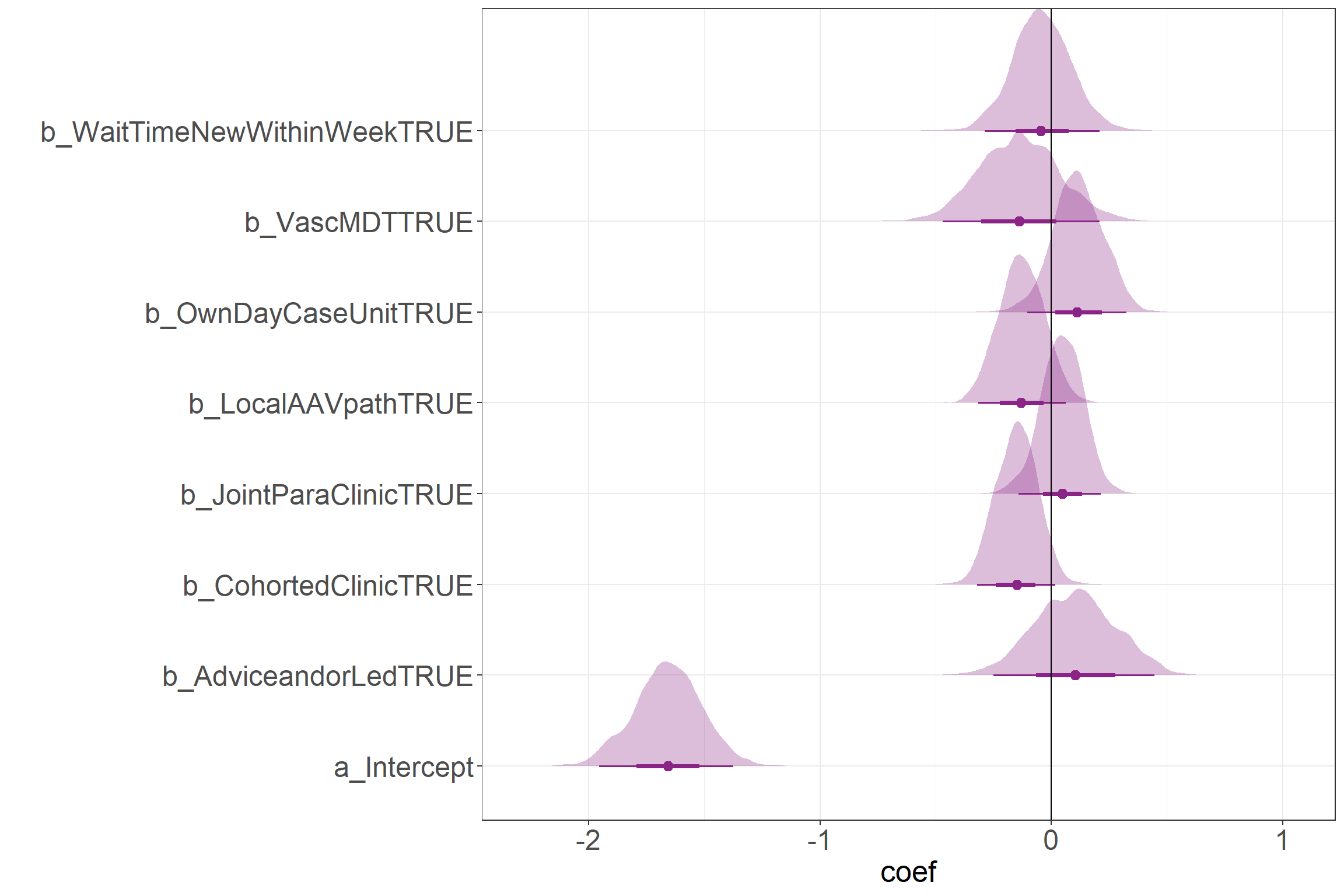
Raw coefficients
This figure shows the raw coefficients on a log scale. With the expection of the Intercept, all values can be compared to the 0 line in order to get a sense for the direction of the effect.
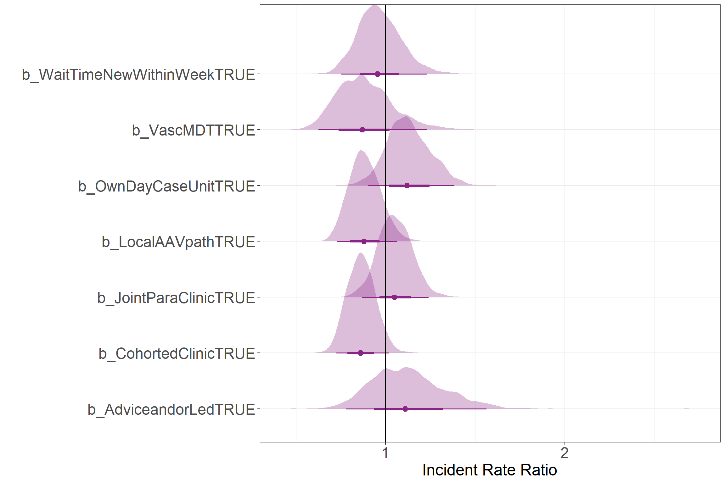
Incident Rate Ratios
This figure shows the Incident Rate Ratio for each service component. These values correspond to the ratio of the rate between a service component being present and not being present. Values greater than one show an increase in the rate, while values lower than one show a decrease in the rate.
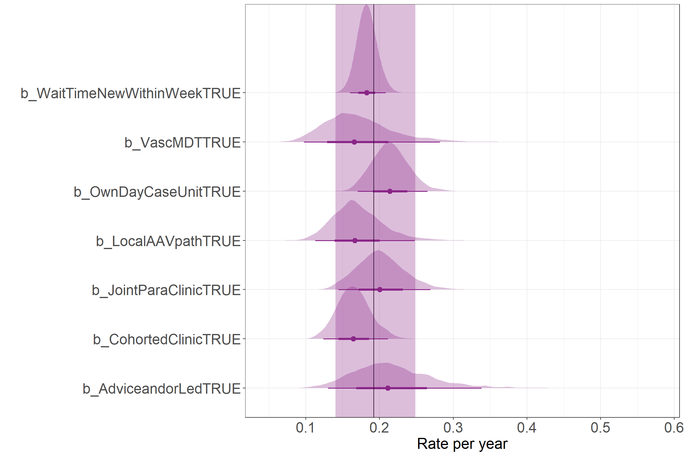
Results as rates
This figure shows the results as rate values. This way compares how the presence of different service components was associated with changes in the yearly rate of Serious Infection. The vertical line represents the mean Intercept rate with the shaded region showing the 95% credibility interval. Please note, this doesn’t show the range of predicted counts, but the uncertainty in the estimate for the mean parameter (i.e., the mean rate of events in these data).
Expected number of events over time
This plot shows the total number of expected events over time in the absence of any of the service components (in grey). Each facet shows how this number of events could be expected to change this count compared to having no other service components. The larger shaded region shows where 95% of the data would be expected to lie in a negative binomial distribution using the point estimates from the model outputs. The solid line shows the mean number of events to be expected given the parameter values. The shaded region between the dashed lines shows the 95% credibility interval around the estimate for the mean value.
# poorly named function... please don't do this, make useful function names
# this function is also really specific to this problem, so it would need to be adapted
# for any other model/dataset
# Using the rnbinom() function is susceptible to the upper and lower bounds moving about due to
# the nature of these data being integers...
makePlot <- function(thisModel, minTime, maxTime, res = .02) {
  post <- thisModel %>% as.matrix() %>%
    as_tibble() %>%
    select(-c(lprior, lp__)) %>%
    mutate(across(2:(ncol(.) - 1), ~ .x + b_Intercept),
           across(1:(ncol(.) - 1), ~ exp(.x))) %>%
    gather(1:(ncol(.)),
           key = "param",
           value = "coef") %>%
    group_by(param) %>%
    mean_hdci(coef)  %>%
    expand_grid(time = seq(minTime, maxTime, res)) %>%
    group_by(param) %>%
    mutate(iter = row_number()) %>%
    select(iter, everything()) %>%
    ungroup()

  quantile_data <- post %>%
    select(param, coef, time) %>%
    spread(param, coef) %>%
    gather(2:(ncol(.) - 1),
           key = "param",
           value = "mu") %>%
    mutate(param = str_remove(param, "b_"),
           param = str_remove(param, "TRUE"),
           q.5 = qnbinom(.5, shape * time, mu = mu * time),
           q.975 = qnbinom(.975, shape * time, mu = mu * time),
           q.025 = qnbinom(.025, shape * time, mu = mu * time))

  mu_post <- post %>%
    select(-c(.width, .point, .interval)) %>%
    filter(!param %in% c("shape", "b_Intercept")) %>%
    left_join(post %>%
                filter(param == "shape") %>%
                select(iter, coef) %>%
                rename(shape = coef)) %>%
    mutate(param = str_remove(param, "b_"),
           param = str_remove(param, "TRUE"),
           q.5_med = qnbinom(.5, shape * time, mu = coef * time),
           q.5_upr = qnbinom(.5, shape * time, mu = .upper * time),
           q.5_lwr = qnbinom(.5, shape * time, mu = .lower * time))

  quantile_data[quantile_data$param != "Intercept",] %>%
    ggplot(aes(time, q.5, colour = param)) +
    geom_path(data = quantile_data[quantile_data$param == "Intercept",] %>%
                select(-param),
              aes(time, q.5),
              colour = "black") +
    geom_ribbon(data = quantile_data[quantile_data$param == "Intercept",] %>%
                select(-param),
                aes(ymin = q.025, ymax = q.975),
                fill = "black",
                colour = "transparent",
                alpha = .1) +
    geom_path() +
    geom_ribbon(aes(ymin = q.025, ymax = q.975,
                    fill = param),
                colour = "transparent",
                alpha = .2) +
    geom_ribbon(data = mu_post,
                aes(x = time,
                    ymin = q.5_lwr - .2, ymax = q.5_upr + .2,
                    y = q.5_med,
                    fill = param),
                alpha = .2,
                linetype = "longdash") +
    scale_x_continuous("Time since Index Date") +
    scale_y_continuous("Estimated total number of Serious Infections") +
    facet_wrap(~param) +
    theme(legend.position = "bottom",
          panel.grid.major.y = element_line())

  # return(post)
}

makePlot(m_nbinom, .1, 24)
Joining with `by = join_by(iter)`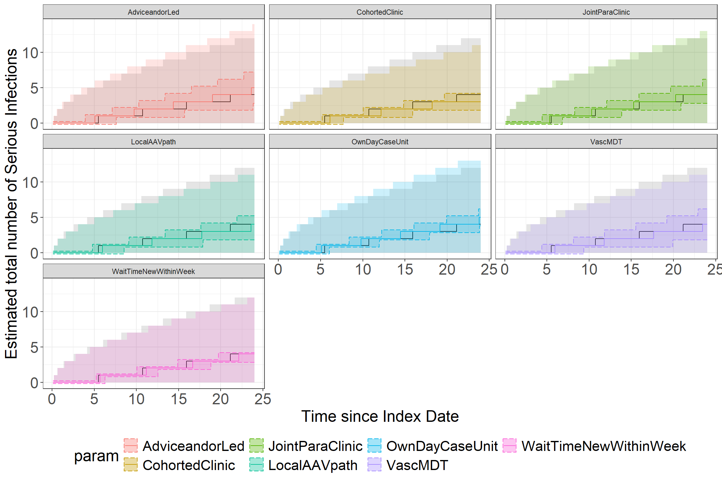
Session Info
sessionInfo()R version 4.3.0 (2023-04-21 ucrt)
Platform: x86_64-w64-mingw32/x64 (64-bit)
Running under: Windows 10 x64 (build 19045)
Matrix products: default
locale:
[1] LC_COLLATE=English_United Kingdom.utf8
[2] LC_CTYPE=English_United Kingdom.utf8
[3] LC_MONETARY=English_United Kingdom.utf8
[4] LC_NUMERIC=C
[5] LC_TIME=English_United Kingdom.utf8
time zone: Europe/London
tzcode source: internal
attached base packages:
[1] stats graphics grDevices utils datasets methods base
other attached packages:
[1] reactable_0.4.4 ggridges_0.5.4 see_0.8.0 brms_2.20.4
[5] Rcpp_1.0.11 tidybayes_3.0.6 lubridate_1.9.2 forcats_1.0.0
[9] stringr_1.5.0 dplyr_1.1.3 purrr_1.0.2 readr_2.1.4
[13] tidyr_1.3.0 tibble_3.2.1 ggplot2_3.5.0 tidyverse_2.0.0
loaded via a namespace (and not attached):
[1] gridExtra_2.3 inline_0.3.19 rlang_1.1.3
[4] magrittr_2.0.3 matrixStats_1.3.0 compiler_4.3.0
[7] loo_2.6.0 callr_3.7.3 vctrs_0.6.5
[10] reshape2_1.4.4 pkgconfig_2.0.3 arrayhelpers_1.1-0
[13] crayon_1.5.2 fastmap_1.1.1 backports_1.4.1
[16] ellipsis_0.3.2 labeling_0.4.3 utf8_1.2.4
[19] threejs_0.3.3 promises_1.2.1 rmarkdown_2.24
[22] markdown_1.8 tzdb_0.4.0 ps_1.7.6
[25] bit_4.0.5 xfun_0.40 jsonlite_1.8.8
[28] later_1.3.1 parallel_4.3.0 prettyunits_1.1.1
[31] R6_2.5.1 dygraphs_1.1.1.6 stringi_1.7.12
[34] StanHeaders_2.26.28 estimability_1.4.1 rstan_2.26.23
[37] knitr_1.43 zoo_1.8-12 base64enc_0.1-3
[40] bayesplot_1.10.0 httpuv_1.6.11 Matrix_1.6-1.1
[43] igraph_2.0.1.1 timechange_0.2.0 tidyselect_1.2.0
[46] rstudioapi_0.15.0 abind_1.4-5 yaml_2.3.7
[49] codetools_0.2-19 miniUI_0.1.1.1 processx_3.8.4
[52] pkgbuild_1.4.2 lattice_0.21-8 plyr_1.8.8
[55] shiny_1.7.5 withr_3.0.0 bridgesampling_1.1-2
[58] posterior_1.5.0 coda_0.19-4 evaluate_0.21
[61] archive_1.1.6 RcppParallel_5.1.7 ggdist_3.3.0
[64] xts_0.13.1 pillar_1.9.0 tensorA_0.36.2.1
[67] checkmate_2.3.1 DT_0.29 stats4_4.3.0
[70] shinyjs_2.1.0 distributional_0.4.0 generics_0.1.3
[73] vroom_1.6.3 hms_1.1.3 rstantools_2.3.1.1
[76] munsell_0.5.0 scales_1.3.0 gtools_3.9.4
[79] xtable_1.8-4 glue_1.7.0 emmeans_1.8.8
[82] tools_4.3.0 shinystan_2.6.0 colourpicker_1.3.0
[85] mvtnorm_1.2-4 grid_4.3.0 QuickJSR_1.0.6
[88] crosstalk_1.2.0 colorspace_2.1-0 nlme_3.1-162
[91] cli_3.6.2 fansi_1.0.6 svUnit_1.0.6
[94] Brobdingnag_1.2-9 gtable_0.3.4 reactR_0.5.0
[97] digest_0.6.33 farver_2.1.1 htmlwidgets_1.6.2
[100] htmltools_0.5.6 lifecycle_1.0.4 mime_0.12
[103] bit64_4.0.5 shinythemes_1.2.0